TLB Tip 005 - An Interesting Conditional Format

This week's tip is a super interesting technique with ranges in conditional format rules.

Let's begin with a list of 20 names, in column A:

Suppose we want to highlight names that occur 2 times or more.

We can build a rule in our Sheet first, before considering conditional formatting. We need to count how many times a name shows up in the list in the next column. To do that we'll use this COUNTIF formula in cell B2:

=COUNTIF($A$2:$A$21,A3)

Notice how we've put $ signs around the range reference $A$2:$A$21 so that it's locked (called an absolute reference). This is important for conditional formatting.

Next, we want to check if this count is greater than 2, because that would indicate a name that occurs more than 2 times.

Add a simple test to make it a conditional and put this formula into the next cell:

=COUNTIF($A$2:$A$21,A3)>2

In the Sheet, we can see the name "Sophia" occurs 3 times, so the formula shows TRUE for those instances:

Now that we have a formula that outputs a TRUE/FALSE, we are ready to create our conditional formatting.

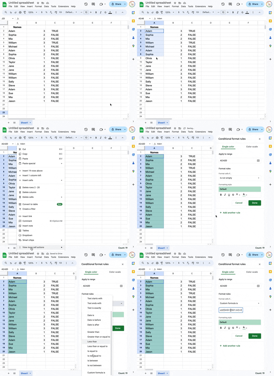
Follow along with the short video clip at the bottom! Here are the steps written below:

Add the conditional formatting rule as follows:

1. Highlight the range containing the 20 names in column A
2. Go to the menu: Format > Conditional Formatting
3. Check that the "Apply to Range" is set to A2:A21
4. For the "Format cells if..." format rule, select the last option in the dropdown: Custom formula is Copy and paste in our formula:
   ​​
   =COUNTIF($A$2:$A$21,A2)>3
5. Change the formatting styles to your desire.
6. Click Done

This will highlight any names (or values) that occur 2 times or more in the list:

Job Well Done!